Fair Lending Lab
Statistical inference Public mortgage dataHypothesis testing on CFPB HMDA mortgage application data. Five hypotheses are defined in the project's registry. H1 was later re-estimated with logistic regression controls: the raw denial-rate gap is +10.7 percentage points, and 44.4 percent remains after adjustment for debt-to-income, combined loan-to-value, loan amount, property value, and income.
Evidence
Screenshots from the live dashboard against Massachusetts 2023 HMDA LAR data.
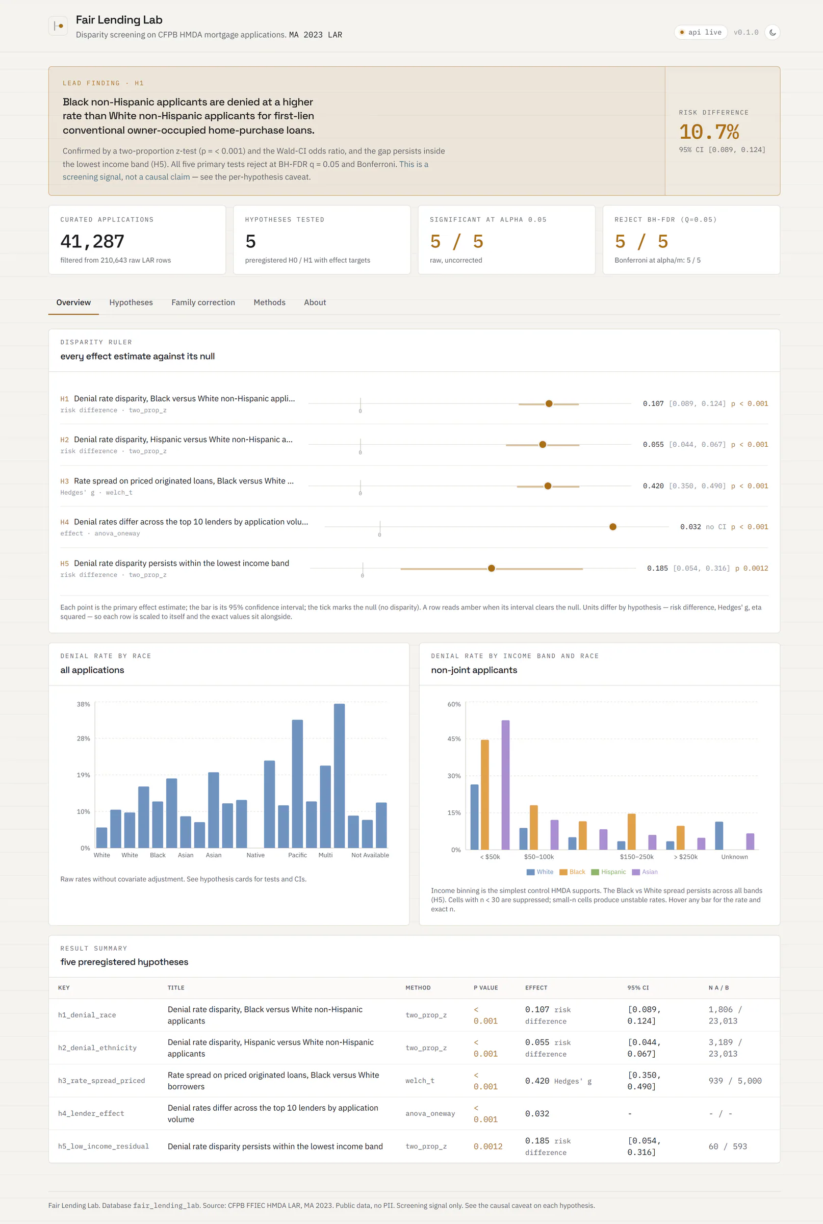
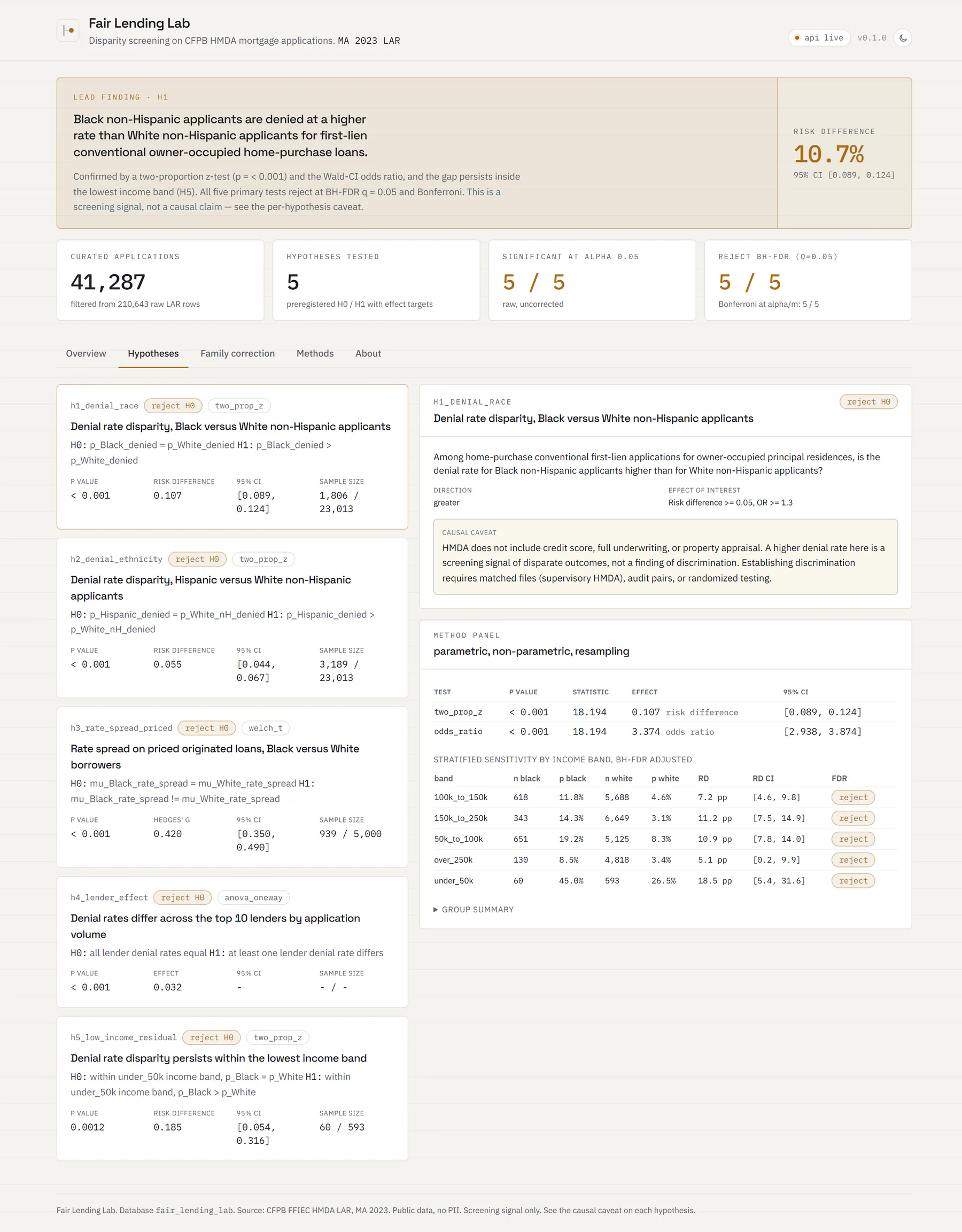
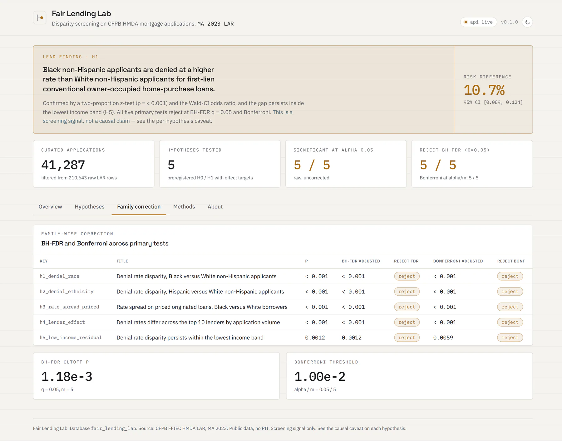
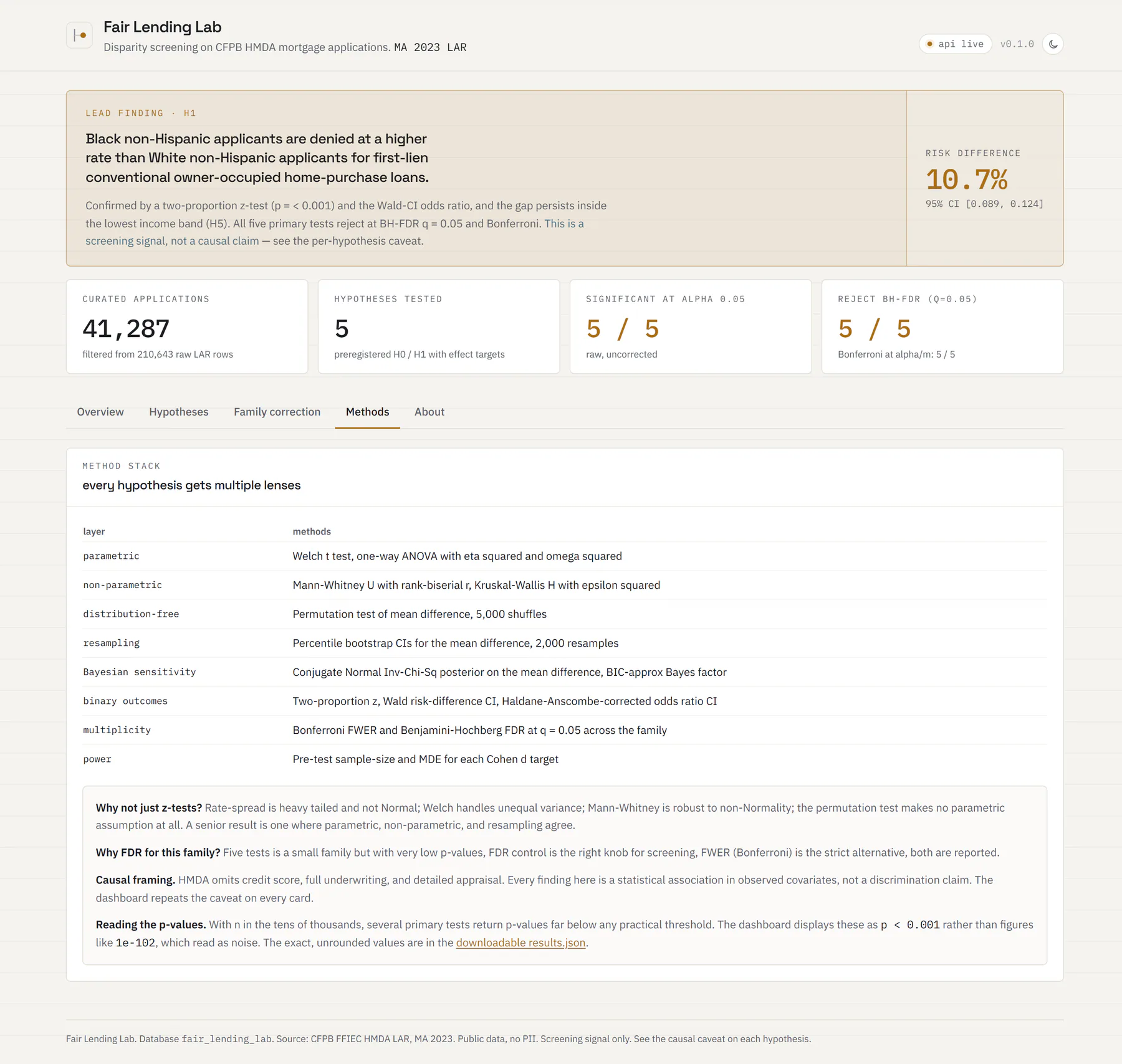

Five hypothesis-driven analyses, with H4 provisional and H5 exploratory
Observations from the scored Massachusetts 2023 prototype. These are screening signals in observed covariates, not findings of discrimination. See the causal framing section below.
- H1 race disparity, raw. Black non-Hispanic applicants face a risk difference of +10.7 percentage points (95% CI 8.9 to 12.4) versus White non-Hispanic applicants for first-lien conventional owner-occupied home-purchase loans (two-proportion z = 18.194, p = 2.9e-74). Stratified by broad income band with BH-FDR adjustment, the raw disparity is positive in every included band.
- H1 race disparity, adjusted. Controlling for debt-to-income, combined loan-to-value, loan amount, property value, and income, the gap falls to +4.73 percentage points (95% CI 3.16 to 6.29), an odds ratio of 2.41 (95% CI 1.96 to 2.95). 44.4 percent of the raw gap survives adjustment (lender-cluster bootstrap 95% CI 32.6 to 54.2 percent). Adding lender and metro fixed effects takes it to +3.55 pp, or 33.3 percent surviving. See the adjusted-model section below.
- H2 ethnicity disparity. Hispanic applicants face a +5.5 percentage point risk difference (95% CI 4.4 to 6.7) versus White non-Hispanic applicants (two-proportion z, p < 0.001). This one has not yet been re-estimated with controls; only H1 has.
- H3 rate spread on priced loans. Among priced originated loans, Black borrowers carry a higher mean rate spread than White borrowers, Hedges g = 0.42 (95% CI 0.35 to 0.49), Welch t p = 6.3e-22. The same direction is reported by Mann-Whitney, a 5,000 permutation test, and a conjugate Bayesian sensitivity.
- H4 lender comparison. In the current unadjusted prototype, denial rates vary across the top 10 lenders. Pairwise two-proportion z tests are reported with BH-FDR and Bonferroni adjustment, but the omnibus ANOVA is provisional and applicant mix is not controlled.
- H5 low-income subgroup. Within the lowest income band, under $50,000 applicant income, the unadjusted Black versus White gap is +18.5 percentage points, with a 95% CI from 5.4 to 31.6 and p = 0.001. Residual income differences and other applicant covariates are not modeled, so this is exploratory.
- Multiple-testing correction. The current implementation reports corrected rejections for all five primary tests. H4 should not be treated as validated until its omnibus test is replaced, and H5 remains exploratory.
Problem
The HMDA Loan Application Register is one of the largest public datasets in financial services. Reading it well requires more than a t test. Large samples can make small differences statistically significant, so effect sizes, uncertainty intervals, appropriate outcome models, and causal framing matter more than rejection alone.
The project demonstrates a hypothesis-driven workflow on a sensitive policy dataset: explicit H0 and H1 statements, methods matched to each outcome, multiple-testing controls, effect sizes with confidence intervals, and a clear separation between association and causation.
Users and decisions
Fair-lending and compliance analysts are the intended users. The dashboard helps them screen observed disparities, compare effect size and uncertainty across hypotheses, and decide where matched supervisory data, loan-file review, or further modeling is warranted.
The dashboard is portfolio methodology. It is not a regulatory finding, a discrimination claim against any lender or applicant pool, or a substitute for the matched-data analyses used in actual fair-lending review.
Five hypothesis-driven analyses over 41,287 HMDA applications
A Python backend ingests the CFPB FFIEC HMDA LAR for a chosen state and year, curates first-lien conventional owner-occupied home-purchase applications into a Postgres fact table, and evaluates five defined hypotheses with outcome-specific methods. H1, H2, and H5 use proportion tests; H3 adds rank-based, permutation, bootstrap, and Bayesian sensitivity analyses; H4 remains an exploratory multi-lender comparison pending a binary-outcome omnibus model. Results are cached as JSONB and exposed by a read-only FastAPI service.
A Next.js frontend renders the same data in a clean analyst console: KPI tiles, a lead-finding callout, a disparity-ruler forest plot, per-hypothesis cards with primary and secondary tests, stratified sensitivity tables, a multiple-testing correction view, and a methods tab. Backend deploys to a Linux VPS behind nginx via systemd, frontend deploys to Cloudflare Pages.
Architecture
Data flow
The pipeline pulls a state-year LAR from the CFPB Data Browser CSV endpoint, projects the 99 raw columns down to the 34 needed for analysis, and COPYs the raw rows into a Postgres staging table. A curated SQL step filters to comparable applications and engineers analysis columns (race rollup, ethnicity rollup, income band, loan amount band, priced-loan flag, denial flag).
Each hypothesis pulls its own slice and runs its assigned primary and secondary analyses, then writes assumption checks and the available sample-size or power context to the analysis-runs log. A denormalized result is upserted to the cache, served by the API, and rendered by the dashboard.
Tools used
Key features
- Five hypotheses defined in a registry with explicit H0, H1, direction, and effect-of-interest target.
- Outcome-specific methods: two-proportion tests and odds ratios for H1, H2, and H5; Welch, Mann-Whitney, permutation, bootstrap, and Bayesian sensitivity for H3; and exploratory lender comparisons for H4 pending a binary-outcome omnibus replacement.
- Multiple-testing correction: Benjamini-Hochberg FDR at q = 0.05 and Bonferroni FWER at alpha / m across the five primary tests.
- Stratified sensitivity for the headline H1 across income bands, with BH-FDR adjustment over strata.
- Pairwise two-proportion z tests across lender pairs, with BH-FDR and Bonferroni adjustment. These comparisons remain unadjusted for applicant mix.
- Sample-size and assumption diagnostics are reported where implemented; complete minimum-detectable-effect coverage remains future work.
- Causal framing caveat on every hypothesis: HMDA omits credit score and full underwriting, so reported disparities are screening signals, not findings of discrimination.
- Deterministic seed across NumPy, SciPy, permutation, bootstrap, and pandas sampling; the notebook reproduces bit identically.
- Pytest plus Hypothesis property tests on the stats helpers, plus a registry sanity test that scans hypothesis text for forbidden characters.
- CI workflow that lints with ruff, runs pytest against a real Postgres service, builds the Next.js frontend, and scans the repo for forbidden em or en dashes.
What this analysis can and cannot claim
Appropriate use: portfolio demonstration of hypothesis testing on a real public dataset, including effect-size reporting, outcome-specific testing, multiple-testing correction, and explicit limitation framing.
Inappropriate use: regulatory determinations, discrimination findings against any specific lender, legal claims against any borrower group, or any operational decision that would normally require matched supervisory data plus loan-file audit pairs.
What the analysis can claim. The reported disparities are associations conditional on the HMDA variables observed. The H1 model shows a residual observed association after partial adjustment, but omitted credit-quality variables, selection, and lender mix remain plausible explanations. The analysis can prioritize deeper review; it cannot assign cause.
What it would take to claim discrimination. Matched supervisory HMDA with credit-bureau records, loan-file review, audit-pair testing, or a counterfactual design. None of those are in scope for a public-data portfolio project, which is why every hypothesis card in the dashboard carries the same caveat in plain language.
Controls cut the disparity from +10.7 pp to +4.73 pp
Headline numbers from the live Massachusetts 2023 dataset. Re-runs against any other state or year are a one-line config change.
The adjusted model
The original analysis reported a raw marginal disparity. This is the same comparison with the underwriting variables HMDA actually carries, fitted as a logistic regression on the H1 cohort of 24,819 applications (1,806 Black non-Hispanic, 23,013 White non-Hispanic). Each row adds controls to the row above it.
- Raw, no controls. Risk difference +10.66 pp. Odds ratio 3.374 (95% CI 2.769 to 4.110, cluster-robust across 377 raw lender LEIs). This reproduces the published +10.7 pp.
- Primary specification. Debt-to-income, combined loan-to-value, log loan amount, log property value, log income. Risk difference +4.73 pp (95% CI 3.16 to 6.29). Odds ratio 2.407 (95% CI 1.964 to 2.949). 44.4 percent of the raw gap survives, with a lender-cluster bootstrap 95% CI of 32.6 to 54.2 percent.
- Plus automated underwriting result. +4.88 pp (3.34 to 6.42). 45.8 percent surviving.
- Plus metro fixed effects. +4.38 pp (2.84 to 5.91). 41.1 percent surviving.
- Plus sex and applicant age. +3.72 pp (2.23 to 5.22). 34.9 percent surviving.
- Fullest specification, adding lender fixed effects. +3.55 pp (2.26 to 4.83). 33.3 percent surviving. Lenders with fewer than 50 applications are pooled into a single model level, but all 377 raw lender LEIs remain separate for cluster-robust inference and bootstrap resampling.
Which control does the work. Entered alone, combined loan-to-value leaves 81.0 percent of the gap, income leaves 76.9 percent, and debt-to-income leaves 63.3 percent. Debt-to-income and combined loan-to-value together account for most of the reduction, taking the gap to +4.64 pp on their own. A complete-case sensitivity that drops the 380 rows with any missing control gives +4.67 pp, so the result is not an artifact of imputation.
Reproducing it. From the platform/ directory: PYTHONPATH=. python -m flab.analysis.adjusted_model --csv data/raw/hmda_2023_MA.csv. The bootstrap draws all 377 raw lender LEI blocks with replacement and is seeded, so the interval reproduces exactly. It defaults to 500 replicates and takes about four minutes on the current benchmark machine; pass --n-boot 50 for a fast check. Output is written to data/processed/adjusted_model.json.
Limitations
HMDA omits credit score, full underwriting detail, property appraisal, and post-application history. Massachusetts 2023 is one state-year of one product line. The disparities here are statistical associations, not causal findings.
Restricting H3 to priced originated loans is a conditioning-on-collider risk: the same underwriting that produces a higher denial rate may also push observed borrowers toward the priced segment. The result is informative about the priced-loan population, not about the underlying borrower population.
The original headline was unadjusted, and more tests would not fix that. The +10.7 pp figure is a raw marginal comparison. In the current implementation, H1 uses a two-proportion z test, an odds ratio, and income-band sensitivity checks. Repeating an unadjusted estimand under additional test families would not address omitted-variable bias. The adjusted model above was added for that reason.
Adjustment does not make this causal. HMDA carries no credit score, reserves, appraisal detail, or compensating factors, so the remaining +4.73 pp is a model-dependent residual association, not an estimate or bound on a lender effect. Omitted variables and downstream controls can bias it in either direction. That is why the financials-only specification is primary and the underwriting layer is shown separately.
Decisions and rejected alternatives
Method breadth over covariate adjustment, which was the wrong trade. I initially emphasized a broad range of inferential methods across the project while leaving the headline H1 estimand unadjusted. That demonstrated range, but the decision required covariate adjustment. The logistic model now reported above changed the headline: 44.4 percent of the raw gap remains after the primary controls.
Multiplicity correction that cannot resolve design uncertainty. BH-FDR and Bonferroni do not change the reported rejections, but they cannot repair an unsuitable H4 primary test or make H5 confirmatory. The project does not preserve a record of every subgroup considered before H5 was selected, so H5 is exploratory regardless of its corrected p-value.
A reported p-value was a floating-point artifact. H1 was initially displayed as p < 1e-300 because a tail-probability calculation underflowed. Recomputing from the z statistic gives 2.9e-74. The decision is unchanged, but the corrected finite value is the one reported here.
An unadjusted ANOVA on a binary outcome for H4. ANOVA can compare group means, but it is not the clearest primary model for binary denial data and its assumptions are not the right basis for a senior lender comparison. The pairwise two-proportion z tests remain descriptive. H4 should be re-estimated with a chi-square test or logistic regression, then adjusted for applicant mix before any lender effect is interpreted.
A registry is not an external preregistration. The project defines H0, H1, direction, and effect targets in code, but it does not provide a public timestamp proving those choices preceded data inspection. Because it also does not record all subgroup cuts considered before H5, this page describes the analyses as hypothesis-driven and treats H5 as exploratory.
What I would build next
Add propensity-score and overlap diagnostics to the existing H1 adjustment. Re-estimate H2 and H5 with covariate controls, replace H4's omnibus ANOVA with a binary-outcome model adjusted for applicant mix, and address H3's selection into priced originated loans. Then add multi-year ingest and define any trend analysis before running it.
Want this for your business?
Through Scott Campbell Consulting I take on data cleanup, dashboards and recurring reporting for small businesses and agencies.