Grid Intelligence
Forecasting Public energy dataA live electricity analytics platform that ingests US EIA, European ENTSO-E, and NOAA weather data into a TimescaleDB warehouse, models it with dbt, scores demand anomalies and forecasts, and serves a public dashboard.
Problem
Electricity data is highly useful but scattered across different public sources, regions, schemas, and publish cadences. Demand, generation mix, interchange, weather, and European load data each arrive differently and need a dependable modeled layer before they can support analysis.
The project needed to demonstrate real analytics delivery rather than a static chart gallery: scheduled ingestion, warehouse design, transformations, API delivery, ML scoring, dashboard interaction, operational freshness, and clear limitations.
Users and decisions
Energy analysts and researchers are the intended users. They can compare regional demand, generation mix, interchange, forecasts, anomalies, and source freshness to decide where deeper investigation is warranted.
The dashboard is built for portfolio demonstration using public electricity and weather data. It is not designed for official operations, reliability decisions, trading, or regulatory analysis.
Four public feeds into one modeled warehouse
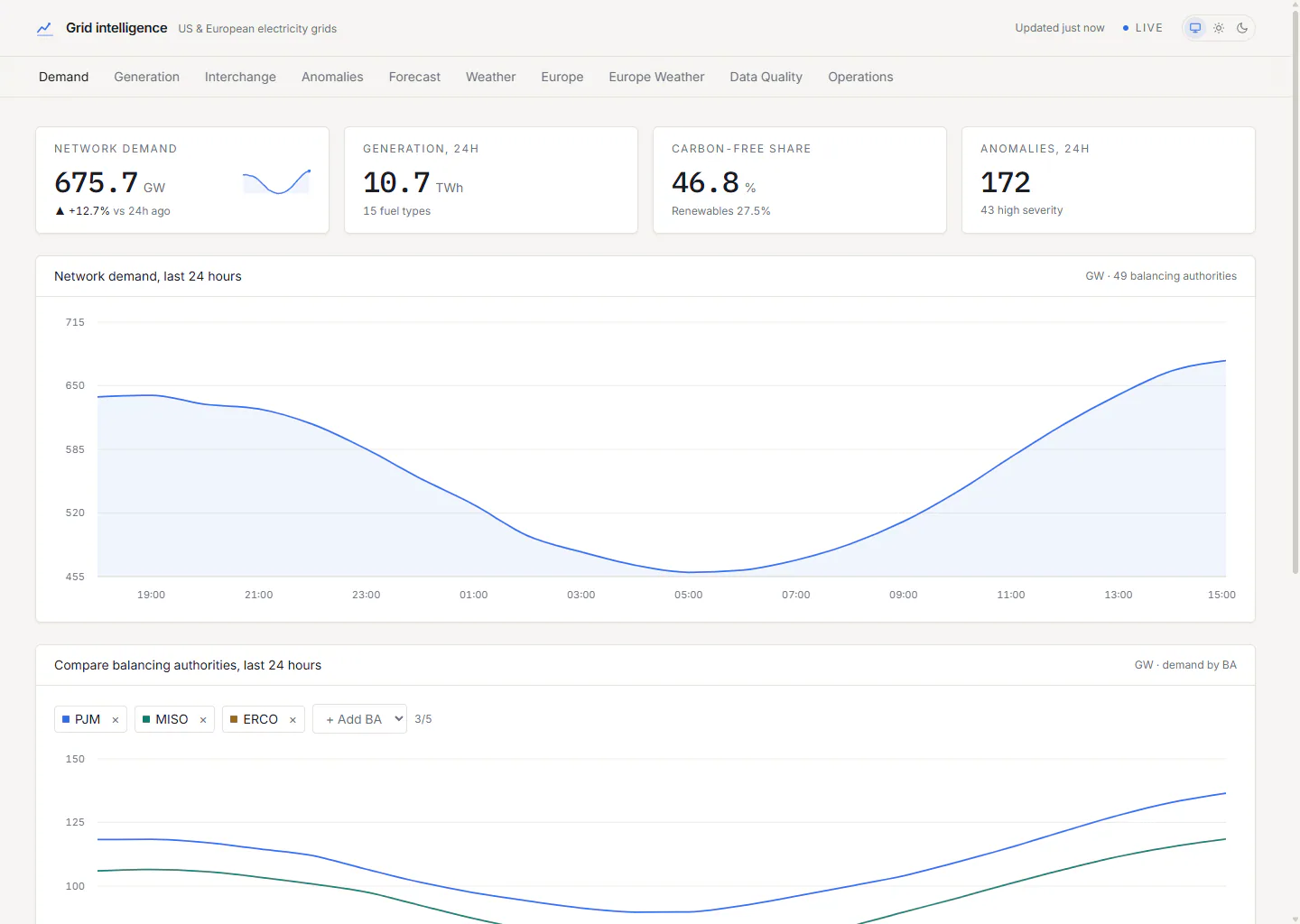
Grid Intelligence runs scheduled ingestion jobs for EIA, ENTSO-E, NOAA, and weather forecast sources, upserts the data into PostgreSQL with TimescaleDB hypertables, models it through dbt, calculates demand forecasts and anomaly scores, and exposes the results through FastAPI and dashboard views.
The same modeled warehouse can feed multiple consumers: a static Next.js dashboard for fast scanning and Power BI-ready mart exports for executive analysis.
Architecture
Data flow
External APIs feed scheduled jobs on their own cadences. Raw observations are stored with natural keys, timestamps, source labels, and update behavior that handles late-arriving facts. dbt models produce demand, generation, interchange, reference, and summary marts with tests around uniqueness, freshness, and expected relationships.
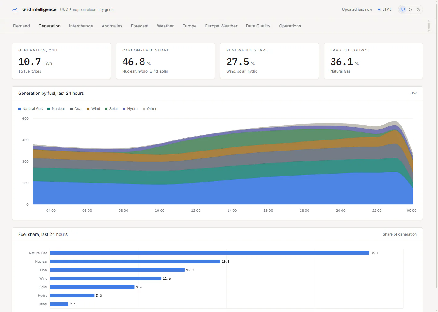
The API layer exposes focused read-only endpoints for headline KPIs, demand history, generation mix, anomaly lists, forecasts, weather, European load, freshness, and health data so presentation code stays separate from data logic.
Tools used
Key features
- Scheduled ingestion for US grid, European grid, and NOAA weather sources.
- TimescaleDB hypertables and dbt models for demand, generation, interchange, weather, and reference data.
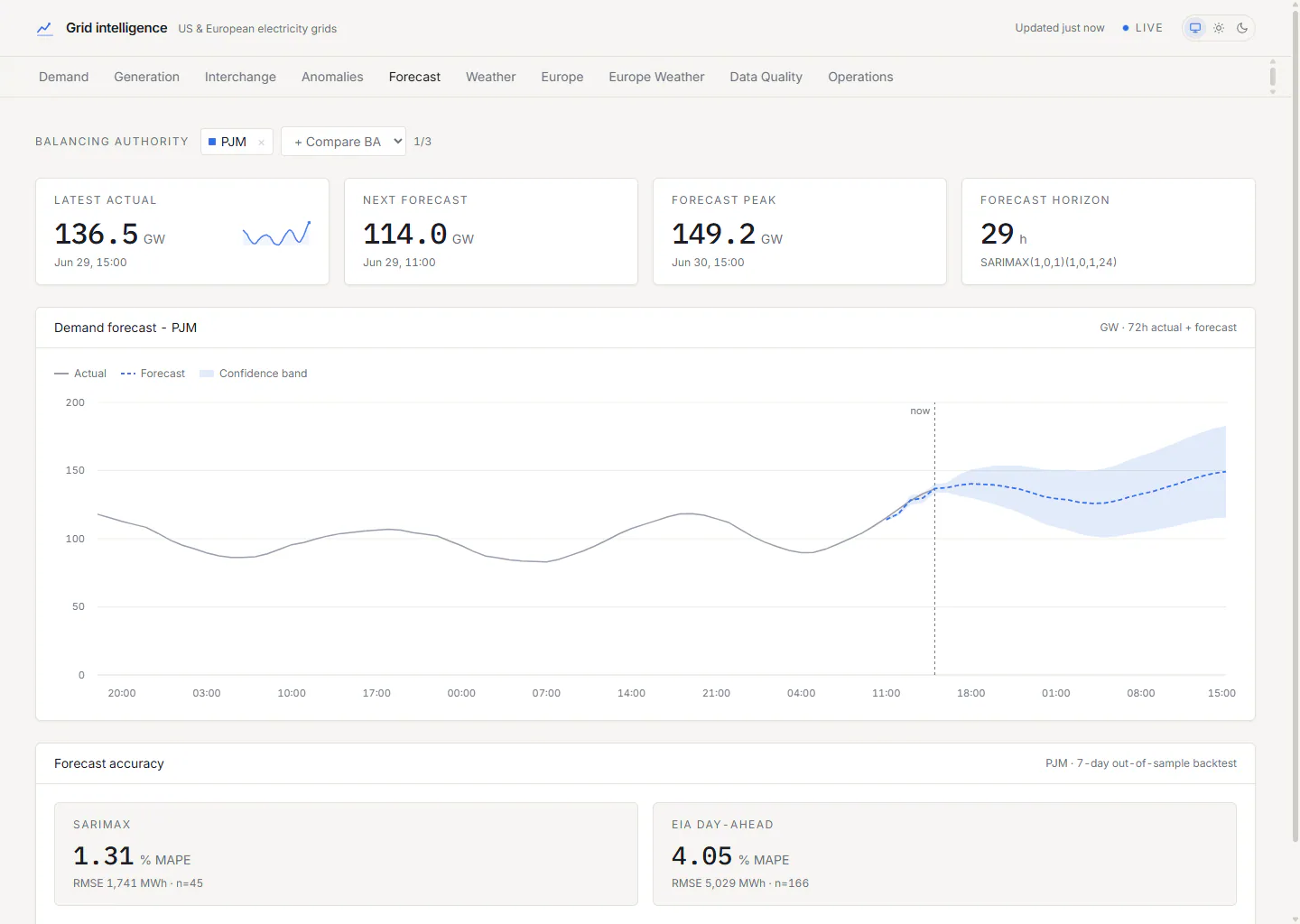
- SARIMAX(1,0,1)(1,0,1,24) day-ahead demand forecasting, scored against the published EIA day-ahead forecast. The seasonal-naive path is a fallback for when the model cannot fit, not the comparison baseline.
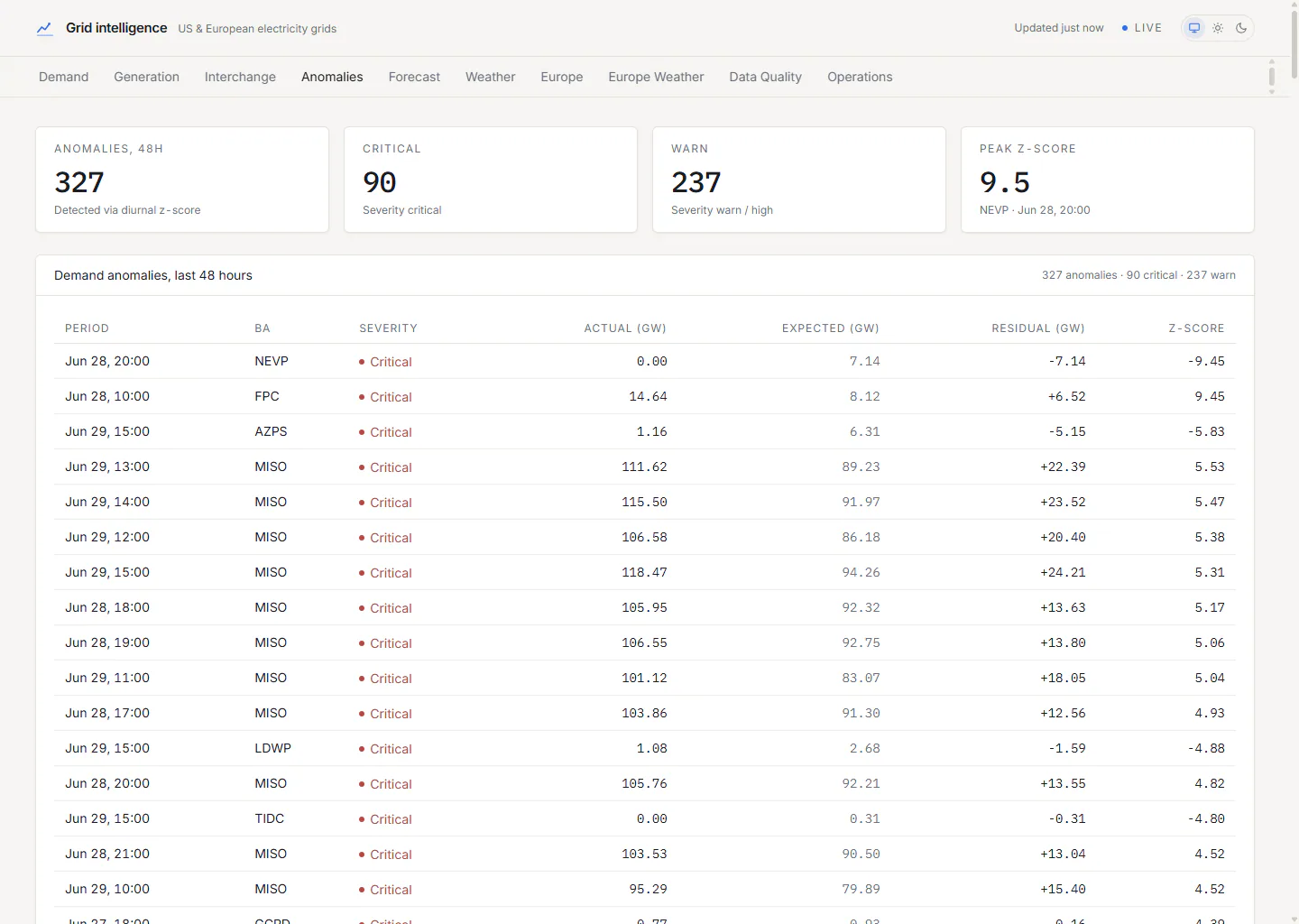
- Diurnal-normalized anomaly scoring with recent anomaly views.
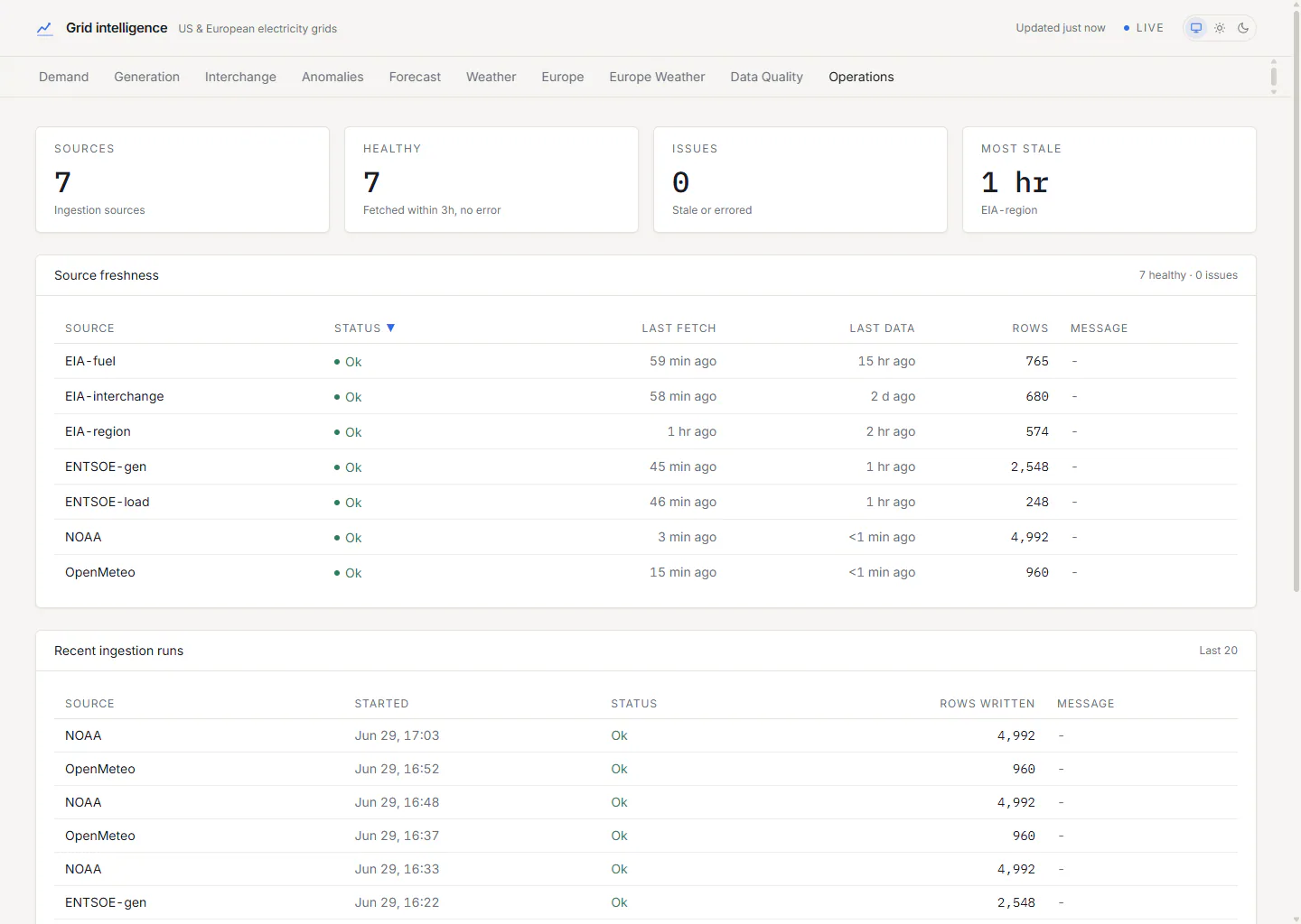
- Dashboard tabs for demand, generation mix, interchange, anomalies, forecast, weather, Europe, data quality, and operations.
- Source freshness and ingestion-run visibility so data reliability is visible.
Tradeoffs and constraints
The project favors transparent public data and reproducible modeling over proprietary feeds or unrestricted operational claims. It tracks many signals, but it does not attempt to replace official grid operators or market systems.
Forecasting and anomaly scoring are demonstration analytics. They show time-series modeling, failure-tolerant ML jobs, and dashboard communication, but they are not official reliability, trading, or planning tools.
Methodology
Appropriate use: portfolio demonstration of public-data engineering, analytics modeling, and dashboard delivery.
Inappropriate use: operational grid decision-making, trading, regulatory analysis, or official reliability assessment.
Forecast skill against a real baseline
The forecast is scored against the day-ahead demand forecast the EIA publishes itself, on the same balancing authorities over the same trailing 168-hour window. That is an operational baseline produced by the system operator, not a naive comparator chosen to be beaten. Both forecasts run at the same horizon: the model is a SARIMAX(1,0,1)(1,0,1,24) issuing predictions 24 hours beyond the last realized actual.
Evidence for
5.49% vs 8.30%Mean absolute percentage error, model against the published EIA day-ahead forecast, across the 48 balancing authorities both cover. A skill score of +33.9 percent.Evidence for
+10.0%RMSE skill over the same set, 1,179 against 1,310 MWh. The gap is far smaller than the MAPE gap, which locates the advantage: the model gains most on small balancing authorities and much less on the large ones that dominate absolute error.Evidence for
35 / 48Balancing authorities where the model records the lower MAPE. It loses on 13, so this is an average advantage rather than a uniform one./v1/forecast/accuracy over a trailing 168 hours, so these figures move. They are a measurement of the running system, not a frozen benchmark.Limitations
The dashboard depends on public source availability, upstream cadence, API keys, and late-arriving revisions. Some records may be delayed, revised, missing, or synthetic when the project is running without live keys.
The project is intentionally scoped as a portfolio analytics system. It should not be treated as an authoritative operational grid system, trading system, or regulatory source.
What the skill score does and does not establish. The comparison is restricted to the 48 balancing authorities both forecasts cover and to a trailing 168-hour window, so the figures move as the window rolls. The two series do not have identical realized-hour counts over that window (8,016 model pairs against 7,532 EIA pairs), so the sets overlap heavily but are not identical. The advantage is also uneven: a +33.9 percent MAPE skill next to a +10.0 percent RMSE skill means most of the gain is on smaller balancing authorities, and the model loses outright on 13 of 48.
What I would improve next
I would add a public API origin for the static frontend path, deeper model evaluation, clearer incident history for ingestion failures, richer European zone labeling, and more documentation around source caveats and transformations.
Want this for your business?
Through Scott Campbell Consulting I take on data cleanup, dashboards and recurring reporting for small businesses and agencies.